
Non-Stationary Structural Causal Bandits
Background
In a stationary environment, the agent can leverage the causal diagram to identify optimal intervention sets—excluding irrelevant variables—that maximize expected reward, and this choice remains valid over time (Lee & Bareinboim, 2018). This works when the environment is fixed for all time steps, as illustrated on the left side of fig. 1.
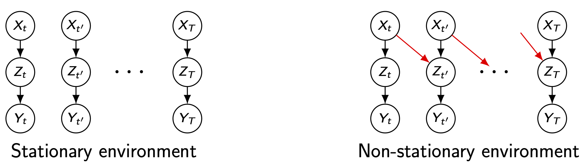 Figure 1
When the world drifts. Under non-stationarity, the same behavior becomes myopic. The reward mechanism and the information that matters can change over time, so yesterday’s optimal arm can degrade today.
What the agent is up against. The hidden data-generating mechanism evolves over time. We analyze it through a time-expanded causal model (i.e., temporal models) whose transition edges encode how information from earlier steps can affect later variables. This changing information flow produces reward disparities across time, which we view as a reward distribution shift given by the intervention history. The key question becomes: which past variables actually transmit useful information to future rewards?
How the agent should act. We reason on a time-expanded causal diagram to separate what changes (reward distribution and effective information flow) from what remains stable. On this basis, we introduce POMIS$^+$—a time-aware extension of POMIS—together with two graphical concepts IB$^+$ and QIB to design non-myopic intervention sequences. Concretely, the agent may intervene on variables that are irrelevant to the current reward but crucial for a future reward via transition edges. This structure-aware strategy clarifies which intervention sets to choose at each time step under reward distribution shifts, effectively identifying the intervention sequence.
Problem setting (NS-SCM-MAB)
Let the bandit environment be generated by a time-indexed SCM (i.e., temporal model) $ \mathcal{M}_t=\langle \mathbf{U}_t,\mathbf{V}_t,\mathcal{F}_t, P(\mathbf{U}_t)\rangle,\ t=1,2,\dots $with reward variable $Y_t\in \mathbf{V}_t$. An arm corresponds to an intervention $ \operatorname{do}(\mathbf{X}_t{=}\mathbf{x}_t) $ on a manipulative set $ \mathbf{X}_t \subseteq \mathbf{V}_t $. Transition edges between time slices encode how variables at time $t$ transmit information to variables at $t{+}1$ (right panel in fig. 1).
A reward distribution shift occurs when the conditional reward distribution changes across time given the intervention history $I_{1:t-1}$: \[ P(Y_t \mid \operatorname{do}(\mathbf{X}_t{=}\mathbf{x}_t), I_{1:t-1}) \neq P(Y_{t’} \mid \operatorname{do}(\mathbf{X}_{t’}{=}\mathbf{x}_{t’}), I_{1:t’-1}) \] Stationary SCM-MAB solutions are myopic here because they optimize $Y_t$ in isolation and ignore cross-time information propagation.
Example
Under the time-slice graph $\mathcal{G}[V_1]$, the agent first computes the MUCT around the current reward $Y_1$ (i.e., ${X_1, Z_1, Y_1}$)
Given this MUCT, the in-slice interventional border (IB) for $Y_1$ is empty. Formally:
\[
\operatorname{MUCT}(\mathcal{G}[V_1],\, Y_1)=\lbrace X_1,\, Z_1,\, Y_1 \rbrace,
\qquad
\operatorname{IB}(\mathcal{G}[V_1],\, Y_1)=\varnothing.
\]
Similarly, another MUCT and IB : \[ \operatorname{MUCT}(\mathcal{G}[V_1]_{\overline{X}_1},\, Y_1)=\lbrace Y_1 \rbrace, \qquad \operatorname{IB}(\mathcal{G}[V_1]_{\overline{X}_1},\, Y_1)=\lbrace Z_1 \rbrace. \]
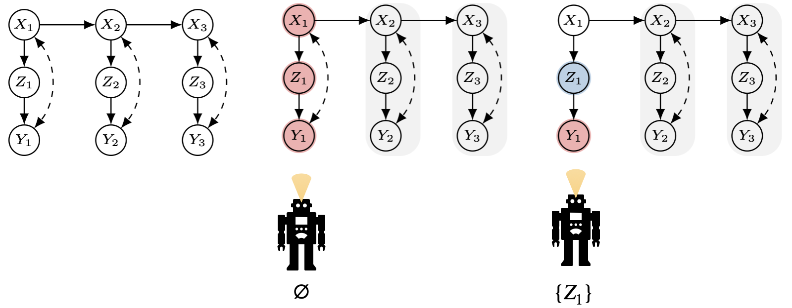 Figure 2
Putting these together, the admissible manipulative sets for $Y_1$ at time $t{=}1$ are the empty set (no intervention needed at the current slice) and the singleton ${Z_1}$ that becomes active once $X_1$ is predetermined. Therefore: \[ \mathrm{POMIS}_1=\lbrace \varnothing, \lbrace Z_1 \rbrace \rbrace \]
Next, suppose the agent computes POMIS at time $t{=}2$.
Given the time slice $\mathcal{G}[V_2]$, the agent obtains the same in-slice family as at $t{=}1$:
\[
\mathrm{POMIS}_2 = \lbrace \varnothing, \lbrace Z_2 \rbrace \rbrace.
\]
However, when the agent chooses the empty set at $t{=}2$, the temporal model it actually faces is
$ \mathcal{M}_2 \mid \mathbf{v}_2^\star{=}x_1$.
The model reflects the influence of a past value at $t{=}1$. Under this conditioning, the local POMIS on $\mathcal{G}[V_2]$ does not guarantee optimality for $Y_2$: the reward at $t{=}2$ can still depend on the prior assignment at $t{=}1$.
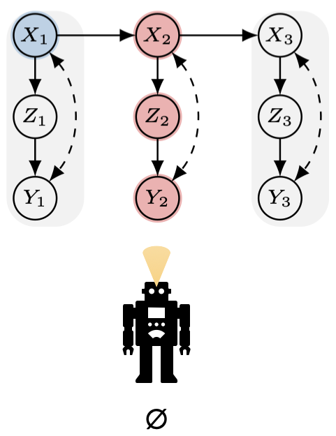
Figure 3
If we widen the view to the rolled-out window $\mathcal{G}[V_1 \cup V_2]$, we see that $X_1$ is the actual POMIS handle for $Y_2$, but it is not intervenable at $t{=}2$. This illustrates why relying only on the in-slice $\mathcal{G}[V_2]$ can be myopic under non-stationarity and motivates using the temporal (cross-time) characterization.
POMIS+ (temporal extension of POMIS)
Single slice (POMIS).
At time $t$, we work on the in-slice graph $\mathcal{G}[V_t]$ for the current reward $Y_t$. We compute the in-slice interventional border $\operatorname{IB}(\mathcal{G}[V_t], Y_t)$. The resulting POMIS at slice $t$ is the family of admissible manipulative sets for $Y_t$ determined by these IB computations.
Graphical tools (IB$^+$ and QIB).
To plan non-myopically toward a future reward $Y_{t’}$ ($t’ > t$), we read the temporal models on the time-expanded diagram:
- IB$^+$ at $t$ toward $t’$ selects the time-$t$ variables that still have leverage on $Y_{t’}$ through transition edges in the rolled-out window. We denote this set by $\mathrm{IB}^{+}_{t,t’}$.
- QIB at $t$ keeps the current-time handles that remain interventional borders for $Y_t$ (under the qualification conditions in the paper). We denote this set by $\mathrm{QIB}_t$.
Composition (definition of POMIS$^+$).
For a given pair $(t,t’)$, the POMIS$^+$ is defined by the union of the two graphical objects:
\[
\mathrm{POMIS}^{+}_{t,t’} \;=\; \mathrm{IB}^{+}_{t,t’}\big(\mathcal{G}[\bigcup_{i=t}^{t’} V_i],\, Y_{t’}\big)
\;\cup\;
\mathrm{QIB}_t\big(\mathcal{G}[V_t],\, Y_t\big).
\]
Under the time-slice Markov assumption used in the paper, it suffices to take $t’ = t{+}1$.
How it’s used (sequence construction).
At each step $t$, we compute $\mathrm{POMIS}^{+}_{t,t+1}$ and select an element $S_t \in \mathrm{POMIS}^{+}_{t,t+1}$.
The overall intervention sequence is then $(S_1, S_2, \dots)$, where each $S_t$ is exactly drawn from the union $\mathrm{IB}^{+}_{t,t+1} \cup \mathrm{QIB}_t$—not an arbitrary set and not based on “including variables irrelevant to $Y_t$” unless they are admitted by the union above.
This is precisely the mechanism we formalized to align current-time leverage with future-time leverage under non-stationarity.
Why stationary solutions fail
In a stationary SCM-MAB, the optimal arm for $Y_t$ is chosen under a fixed reward mechanism. Under reward distribution shift or altered information propagation, a myopic choice may:
- under-exploit transition edges that create leverage on $Y_{t’}$,
- over-explore variables with no lasting effect,
What we demonstrate
- A causal formalization of NS-SCM-MAB with precise reward distribution shift and temporal model semantics.
- A graphical characterization for non-myopic intervention design using IB+ and QIB.
- A constructive method to build POMIS+ intervention sequences that exploit information propagation.
- Experiments showing improved cumulative regret and higher optimal-action probability versus stationary or naive baselines under non-stationarity.